iCite and W2P ratios - new ways of quantifying scientific productivity

What's the best way of ranking scientists based on their productivity?

There are lots of options including:

• number of publications
• number of citations
• impact factor of the journals the publications are in

All have strengths and weaknesses.

Recently, leaders at my academic institution have started to talk publicly about h-indices. These are calculated for each author as the number (x) of publications he/she has that have each been cited at least x times. That's an interesting idea because it rewards impact; people who publish lots of papers that nobody cites have lower h-indices than people who publish a few manuscripts that are very influential. However the h-index has the drawback that it grows with time (because people publish more papers and they have more time to be cited). This means that it favors seasoned scientists who have been productive for a long time. It's not a great way of identifying a rising star.

I don't think that there will ever be a single perfect metric that scientists can use to quantify productivity but I was excited to see that NIH is supporting the Relative Citation Ratio with their new iCite tool.

The Relative Citation Ratio (RCR) is an article level metric that quantifies scientific influence. To quote a help box from iCite, "It is calculated as the cites/year of each paper, normalized to the citations per year received by NIH-funded papers in the same field."

The Weighted RCR is the sum of the individual RCRs for a group of papers.

This creates an interesting opportunity. If you calculate the ratio of the Weighted RCR to Total Publications (I'll call it W2P) you get a single value that defines the influence of a collection of papers.

If your W2P is greater than 1, your papers are more influential than those of your NIH-funded colleagues. If it's less than 1, your papers are being cited less often than average.

WtoP doesn't scale with the number of papers you publish so it shouldn't depend on the length of your career.

Only time will tell how scientists use these new metrics but I am going to make a bold (and probably rash) prediction. Since NIH is supporting RCRs, I think that they will take over from h-indices as the mostly commonly used measure of productivity in US biomedical science.

For the record, here are my current stats

• 46 publications
• h-index = 22
• Weighted RCR = 59.98
• W2P = 1.34

and for the truly nerdy

• Erdos number = 8

Word clouds

A quick aside - I will get back to POV-Ray soon.

I wanted to make a Word Cloud for something at work. I've never done this before so I adopted my usual strategy - look in the MATLAB FileExchange to see if somebody has already created a tool.

As is nearly always the case, I found something useful, WordData Visualization. It was even a Pick of the Week back in 2015.

Five minutes later, and I had what I wanted. Then I went on to generate a figure based on the text from my PhD thesis. It doesn't get much more exciting :-)

Standard errors

This post is going to be about the standard error of the mean, which is often just referred to as the standard error.

As a reminder, we're basing our discussion on a distribution of 5 km race times. The mean of the race times is 25.001 minutes. The standard deviation s is 2.973 minutes. The mean tells you where the distribution is centered. The standard deviation tells you about its width. Look back at the last post if you need a reminder.

The standard error is subtly different. It doesn't really describe your distribution. Rather, it helps you to understand how accurately you know the mean value of your data.

But the mean is the mean, you're thinking. How can it change?

Well, you're right. You calculated the mean of 500 race times. That's a fixed number. But the assumption in this type of statistics is that you're pulling these race times from an infinite series of potential times. When you picked this particular set of 500 values, the mean happened to be 25.001. That's now your estimate of the true mean of the infinite series of potential times.

But you could have picked a different set of 500 race times from the infinite list of potential numbers, in which case, you'd probably have calculated a different estimate of the mean. A third set of 500 times could have given you a still different estimate. And so on ...

How much would these estimates of the true mean vary? That's what the standard error helps you to decide.

Take a look at the histograms below. They show what happens when you split the 500 original race times into groups of different sizes and then calculate the mean of each group.

So the middle panel (group size = 5) shows the distribution of means calculated using 100 groups which each contain 5 race times. The first value represented in the histogram is the mean of the first 5 race times, the second value is the mean of the second 5 race times, and so on.

Do you see how the distributions get narrower as the group size increases? That is because as you include more and more points in the group, it becomes increasingly representative of the original population. By the time you're averaging 20 points, there's not much difference between the individual subsets.

You can calculate the width of the histograms above just like we did when we calculated the standard deviation in the last post. The width of these distributions is the standard error of the mean. It goes down as you increase the group size. You can also calculate it as



from Wikipedia where s is the standard deviation calculated for your samples and n is the number of data points you have. As you increase n, the standard error goes down, because your points are becoming more representative of the original population. However, there are diminishing returns. Once you already have quite a few data points, you have to add a lot more to get a better estimate of the mean. That bit comes from the square root of n on the bottom.

So in summary,

• the mean tells you where your data are centered
• the standard deviation quantifies the spread in your original data
• the standard error describes the uncertainty associated with the mean value

Next up, one-sample t-tests.

Distributions and standard deviations

This post is going to be about distributions and statistics that summarize them.

I run 5 km races fairly often and so do many of my friends. Here are the latest times (in minutes) for a few of us.

23.053, 28.543, 22.725, 21.671, 22.463, 23.282

[Okay, I'm cheating a bit here. You probably realized that we don't time our runs to 3 decimal places. I made these numbers up in MATLAB because I want a concrete example, but bear with me.]

The fastest time in this small group was ~21.7 minutes. The slowest was just over 28.5 minutes. It looks like our average time was ~25 minutes.

The next image shows a histogram for 500 5 km times. (Download the data here if you want to follow along.) The x axis shows the time in minutes. The y axis shows the number of people who ran that time.

If you look at this distribution, you can see that our fastest runner completed his race in 17 minutes (there's a bar of height 1 at 17). Similarly, two of our group took 35 minutes.

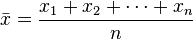
This histogram is centered around 25 minutes. Some of us took less time, some of us took more, but our 'middle time'  was ~25 minutes. You can calculate that by adding up all the 5 km times and dividing by the number of races. Here's the equation copied from Wikipedia.



For our data, the mean happens to be 25.0 minutes.

Knowing the mean value of a distribution is often helpful but it can be useful to know how wide the distribution is too. For example, you might want to know whether (a) we are all run very similar times, or (b) whether our times span a big range. These would correspond to narrow and wide distributions respectively.

The key parameter here is the standard deviation, written as s. The standard deviation for the narrow distribution above is 1. The standard deviation for the wide distribution is 4.

You can calculate the standard deviation using another formula, again copied from the Wikipedia page



However, I think it might be more useful to think about what the standard deviation actually represents.

Take a look at this formula

You can think of this as a constant (the bit before the e) multiplied by e^something.

The e^something bit is the interesting part. (x-µ)² is greater than or equal to zero because squared numbers cannot be negative. Similarly, (2*s²) also has to be greater than or equal to zero.

So the term

is e to the power of 0 (when x is µ) or e to the power of a negative number.

The maximum value of the term is 1 when x is µ. The term heads to zero as x becomes bigger or smaller than µ. If s is big, the term heads to zero slowly. Conversely if s is small, the term drops to zero very quickly as x moves away from µ.

f(x) is the equation for the normal distribution. It's a very important example of a bell-shaped or Gaussian curve. (All Gaussian curves have the functional form e^{-something x2}). The bit at the beginning just makes sure that the area under the curve always equals 1.

You can fit f(x) to our histogram by adjusting the values of µ and s until you get the best possible match between the curve and the data. (We'll talk more in later posts about how to do this fitting.) When you do this

• µ is the mean of the data
• s is the standard deviation

Here's what the fit looks like for our data.

In summary, the mean of a distribution tells you where it is centered. The standard deviation s tells you how wide it is.

Next up, standard errors.

Statistics - introduction

This is the introduction to a series of posts about statistics.

I intend to start slowly and build up to cover one and two-sample t-tests. If things go well, I hope to extend the discussion to linear and non-linear regression. I hope that after reading this series you will be able to explain to your friends what the p value of a regression line means.

My approach is heavily influenced by Harvey Motulsky's book "Intuitive Biostatistics". I highly recommend buying this book, or at least borrowing it from your library and devouring it voraciously. It completely changed the way I think about statistics.

The first post in this series will cover means, standard deviations, and standard errors.