This post is going to be about distributions and statistics that summarize them.
I run 5 km races fairly often and so do many of my friends. Here are the latest times (in minutes) for a few of us.
23.053, 28.543, 22.725, 21.671, 22.463, 23.282
[Okay, I'm cheating a bit here. You probably realized that we don't time our runs to 3 decimal places. I made these numbers up in MATLAB because I want a concrete example, but bear with me.]
The fastest time in this small group was ~21.7 minutes. The slowest was just over 28.5 minutes. It looks like our average time was ~25 minutes.
The next image shows a histogram for 500 5 km times. (Download the data here if you want to follow along.) The x axis shows the time in minutes. The y axis shows the number of people who ran that time.

If you look at this distribution, you can see that our fastest runner completed his race in 17 minutes (there's a bar of height 1 at 17). Similarly, two of our group took 35 minutes.
This histogram is centered around 25 minutes. Some of us took less time, some of us took more, but our 'middle time' was ~25 minutes. You can calculate that by adding up all the 5 km times and dividing by the number of races. Here's the equation copied from Wikipedia.
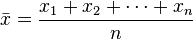
For our data, the mean happens to be 25.0 minutes.
Knowing the mean value of a distribution is often helpful but it can be useful to know how wide the distribution is too. For example, you might want to know whether (a) we are all run very similar times, or (b) whether our times span a big range. These would correspond to narrow and wide distributions respectively.

The key parameter here is the standard deviation, written as s. The standard deviation for the narrow distribution above is 1. The standard deviation for the wide distribution is 4.
You can calculate the standard deviation using another formula, again copied from the Wikipedia page

However, I think it might be more useful to think about what the standard deviation actually represents.
Take a look at this formula

You can think of this as a constant (the bit before the e) multiplied by esomething.
The esomething bit is the interesting part. (x-µ)2 is greater than or equal to zero because squared numbers cannot be negative. Similarly, (2*s2) also has to be greater than or equal to zero.
So the term

is e to the power of 0 (when x is µ) or e to the power of a negative number.
The maximum value of the term is 1 when x is µ. The term heads to zero as x becomes bigger or smaller than µ. If s is big, the term heads to zero slowly. Conversely if s is small, the term drops to zero very quickly as x moves away from µ.
f(x) is the equation for the normal distribution. It's a very important example of a bell-shaped or Gaussian curve. (All Gaussian curves have the functional form e-something x2). The bit at the beginning just makes sure that the area under the curve always equals 1.
You can fit f(x) to our histogram by adjusting the values of µ and s until you get the best possible match between the curve and the data. (We'll talk more in later posts about how to do this fitting.) When you do this
Here's what the fit looks like for our data.

In summary, the mean of a distribution tells you where it is centered. The standard deviation s tells you how wide it is.
Next up, standard errors.
I run 5 km races fairly often and so do many of my friends. Here are the latest times (in minutes) for a few of us.
23.053, 28.543, 22.725, 21.671, 22.463, 23.282
[Okay, I'm cheating a bit here. You probably realized that we don't time our runs to 3 decimal places. I made these numbers up in MATLAB because I want a concrete example, but bear with me.]
The fastest time in this small group was ~21.7 minutes. The slowest was just over 28.5 minutes. It looks like our average time was ~25 minutes.
The next image shows a histogram for 500 5 km times. (Download the data here if you want to follow along.) The x axis shows the time in minutes. The y axis shows the number of people who ran that time.

If you look at this distribution, you can see that our fastest runner completed his race in 17 minutes (there's a bar of height 1 at 17). Similarly, two of our group took 35 minutes.
This histogram is centered around 25 minutes. Some of us took less time, some of us took more, but our 'middle time' was ~25 minutes. You can calculate that by adding up all the 5 km times and dividing by the number of races. Here's the equation copied from Wikipedia.
For our data, the mean happens to be 25.0 minutes.
Knowing the mean value of a distribution is often helpful but it can be useful to know how wide the distribution is too. For example, you might want to know whether (a) we are all run very similar times, or (b) whether our times span a big range. These would correspond to narrow and wide distributions respectively.

The key parameter here is the standard deviation, written as s. The standard deviation for the narrow distribution above is 1. The standard deviation for the wide distribution is 4.
You can calculate the standard deviation using another formula, again copied from the Wikipedia page
However, I think it might be more useful to think about what the standard deviation actually represents.
Take a look at this formula

The esomething bit is the interesting part. (x-µ)2 is greater than or equal to zero because squared numbers cannot be negative. Similarly, (2*s2) also has to be greater than or equal to zero.
So the term

is e to the power of 0 (when x is µ) or e to the power of a negative number.
The maximum value of the term is 1 when x is µ. The term heads to zero as x becomes bigger or smaller than µ. If s is big, the term heads to zero slowly. Conversely if s is small, the term drops to zero very quickly as x moves away from µ.
f(x) is the equation for the normal distribution. It's a very important example of a bell-shaped or Gaussian curve. (All Gaussian curves have the functional form e-something x2). The bit at the beginning just makes sure that the area under the curve always equals 1.
You can fit f(x) to our histogram by adjusting the values of µ and s until you get the best possible match between the curve and the data. (We'll talk more in later posts about how to do this fitting.) When you do this
- µ is the mean of the data
- s is the standard deviation
Here's what the fit looks like for our data.

In summary, the mean of a distribution tells you where it is centered. The standard deviation s tells you how wide it is.
Next up, standard errors.
No comments:
Post a Comment