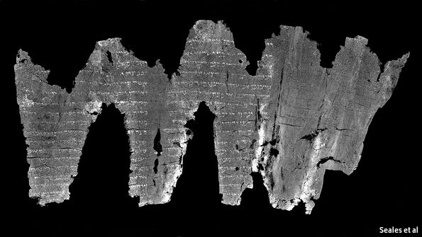
How to read things without opening them

Brent Seales is a professor of computer science at the University of Kentucky. He drives several very cool research programs in areas ranging from robotic surgery to advanced image progressing.

Recently, the Economist (one of my favorite weekly reads) featured some of his work. Here's a link.

How to read an old scroll without opening it

Filtering binary images by object size in MATLAB

As usual, I learned something new when I read Steve Eddin's latest blog post.

This time around, I discovered that MATLAB has some new features that make it easy to filter binary objects based on their size. There were, of course, old ways to do this but the new bwareafilt command (at least, new in MATLAB 2014B) simplifies some workflows.

Update on WTFIT

A few weeks ago I blogged about an amazing new bot that was developed by the incomparable Ming Cheuk.

Since then, I've been wondering exactly how it works. Ming's interesting post on Medium provides some answers.

Finally, just for the record, and to keep things in perspective, I should point that WTFIT doesn't always work exactly like you'd hope.

Here's a picture I tested it with. The main character in the image is Ming.

Image recognition and a new bot

Ming Cheuk, an exceptionally talented PhD student at the University of Auckland, has created a bot to identify objects in pictures. He calls it WTFIT.

I thought I'd give it a try. You just log in with Facebook and send it a picture. Here's what I got.

Amazing. Try it yourself at http://www.wtfitbot.com/

New options for thresholding images in MATLAB

I've written several posts recently about thresholding images. I was thus pretty excited to see Steve Eddins announce a new series of posts on his blog.

http://blogs.mathworks.com/steve/2016/04/28/image-binarization-new-functional-designs/

My impression from a very quick scan of the documentation is that MATLAB 2016a includes a new function imbinarize which can be called with a locally adaptive threshold option.

I don't think this will lead to a breakthrough in image processing - adaptive thresholding is not a new technique - but it will simplify coding. The new function will allow users to replace multiple lines of 'old' MATLAB code with a single command.

And in my opinion, that's why MATLAB is so useful for scientific computing. It's not that the software gives you completely new options; you can code anything in C if you want to. It's just that MATLAB makes it easy to try things without investing huge amounts of time. That's why it accelerates science.

Image segmentation - part 3

This is the third post in our discussion of image segmentation. The first post talked about splitting an image by RGB color using ImageJ / Fiji. Then I talked about using k-means segmentation and the L*a*b color space. You might remember that I was pretty excited about the technique. Is it a general solution to all segmentation problems?

Let's try it on this image.

When I look at this picture, I see 3 colors: white, black/blue and lots of red. Let's convert from RGB to L*a*b and then split into 3 regions using k-means segmentation. The MATLAB code to do this is

function k_means_clustering

image_file_string = '3mokotri.tif';

% Load image

im_rgb = imread(image_file_string);

% Transform to lab color space

cform = makecform('srgb2lab');

im_lab = applycform(im_rgb,cform);

% Create a n x 2 matrix of [a b] values

a = im_lab(:,:,2);

a = double(a(:));

b = im_lab(:,:,3);

b = double(b(:));

ab = [a b];

% Construct the 2D histogram with appropriate limits

c{1}=[min(ab(:)) : max(ab(:))];

c{2}=c{1};

n = hist3(ab,c);

n1 = n';

n1(size(n,1) + 1, size(n,2) + 1) = 0;

% Display

figure(1);

clf;

imagesc(log10(n1));

hold on;

title('2D histogram of pixel values, colored based on log10 of pixel count')

xlabel('a value');

ylabel('b value');

[id,cl]=kmeans(ab,3);

figure(2);

clf;

hold on;

cm = paruly(3);

for i=1:3

    vi = find(id==i);

    plot(ab(vi,1),ab(vi,2),'+','Color',cm(i,:));

    plot(cl(i,1),cl(i,2),'md','MarkerFaceColor','m');

end

xlabel('a value');

ylabel('b value');

set(gca,'YDir','reverse');

[r,c] = size(im_rgb(:,:,1));

im_cluster = reshape(id,r,c);

figure(3);

imagesc(im_cluster);

The end result is

Hmm, that was not what I was hoping for.

Compare with the original again.

It looks like the algorithm did a good job of finding the white lines but it didn't find the black dots I was looking for. Instead, it separated the red areas in the original picture into dark red and light red (maybe pink?) areas.

I have some ideas about how to improve the algorithm for this particular image (which I intend to address in future posts) but I think I've just demonstrated a general result of image processing. It's hard to find a single approach that works for every type of task. It's also hard to develop techniques that don't have a few fiddle factors (parameters that you adjust until 'something works').

Image processing is never easy but as you gain experience and learn more about the techniques that are available, you begin to make faster progress.

Next up, some thoughts on t-tests.

Image segmentation - part 2

This continues the previous post where we talked about segmenting a test image into 3 parts. As a reminder, here's the test image again.

k-means clustering takes your data points and tries to group them into k clusters. It's a general technique that can be used with many sorts of data but it can be useful for segmenting images.

If you want to segment by color, it's often easier to switch to the L*a*b color-space. When you do this, the second and third planes contain all of the color data. The first L plane is to do with brightness.

Here's some MATLAB code that

1. loads our test image
2. transforms it into the lab color space
3. calculates the 2D histogram of pixel intensities
4. displays the heat map of the histogram with a log color scale

function k_means_clustering

image_file_string = 'hubert_8_3_small.png';

% Load image

im_rgb = imread(image_file_string);

% Transform to lab color space

cform = makecform('srgb2lab');

im_lab = applycform(im_rgb,cform);

% Create a n x 2 matrix of [a b] values

a = im_lab(:,:,2);

a = double(a(:));

b = im_lab(:,:,3);

b = double(b(:));

ab = [a b];

% Construct the 2D histogram with appropriate limits

c{1}=[min(ab(:)) : max(ab(:))];

c{2}=c{1};

n = hist3(ab,c);

n1 = n';

n1(size(n,1) + 1, size(n,2) + 1) = 0;

% Display

figure(1);

clf;

imagesc(log10(n1));

hold on;

title('2D histogram of pixel values, colored based on log10 of pixel count')

xlabel('a value');

ylabel('b value');

The output is

When I look at the test image, I see three colors: a gray/white that forms the background, an orangey-yellow that is muscle tissue, and a darker red that indicates collagen. So let's try to split the pixel values into 3 separate groups. In MATLAB, the command is

[id,cl]=kmeans(ab,3);

id is a vector with values of 1,2, or 3. These link each pixel to a given cluster.
cl is a 3x2 array which shows the centroids of the clusters.

This snippet of code shows which [a,b] values fall into each cluster. The magenta markers show the centroids (cl) of each cluster.

figure(2);
clf;
hold on;
cm = paruly(3);
for i=1:3
    vi = find(id==i);
    plot(ab(vi,1),ab(vi,2),'+','Color',cm(i,:));
    plot(cl(i,1),cl(i,2),'md','MarkerFaceColor','m');
end

set(gca,'YDir','reverse');

giving

It's now easy to set each pixel in the original image based on it's cluster identity. You just have to reshape the id vector.

[r,c] = size(im_rgb(:,:,1));
im_cluster = reshape(id,r,c);

figure(3);
imagesc(im_cluster);

The output is

Compare this result to the original.

The segmentation is not perfect but we didn't set any parameters other than 'we want 3 colors'. It's also super-fast and objective. I think it's pretty cool.

Is k means clustering a perfect solution for image segmentation? We will look at that in the next post.

Image segmentation, part 1

I often want to calculate numbers that quantify features in images. For example, the picture below is a cross-section of a piece of heart muscle. The edges are mostly white/gray and are the background of the slide. The light orange parts are muscle. The red parts are collagen.

I want to calculate the relative content of collagen, that is the number of pixels that are collagen divided by the number of pixels that aren't background.

When my lab has done this in the past, we've segmented the image by thresholding in the RGB plane. The screenshot below shows an initial attempt using the Color Thresholding tool in Fiji.

I think this approach works, eventually, but it requires a lot of fiddling to get the thresholds right, and it's definitely subjective. When I came across this page in the MATLAB documentation, I wondered if k-means clustering might be a better option.

We'll describe that approach in the next post.